


Introduction:
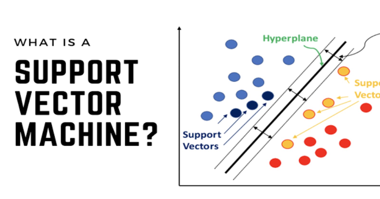
Support Vector Machines (SVM) represent a class of supervised machine learning algorithms widely recognized for their efficacy in classification and regression tasks. At its essence, SVM seeks to delineate decision boundaries in a high-dimensional space to classify data points into different categories or predict continuous numerical values. The core principle behind SVM is to identify the optimal hyperplane that separates instances of distinct classes while maximizing the margin, which is the distance between the hyperplane and the nearest data points of each class, known as support vectors.
In classification tasks, SVM endeavors to find the hyperplane that best segregates the data points into distinct classes. This hyperplane serves as a decision boundary, facilitating the classification of new instances based on their features. SVM employs various kernel functions, such as linear, polynomial, and radial basis function (RBF), to map the input data into a higher-dimensional space where the classes become linearly separable. By maximizing the margin, SVM enhances robustness against noise and generalizes well to unseen data, thereby mitigating overfitting.
Furthermore, SVM can also be applied to regression tasks, where the objective is to predict continuous numerical values. In regression, SVM constructs a hyperplane that captures the relationship between the input features and the target variable, with the aim of minimizing the prediction error. By leveraging the principles of margin maximization and support vectors, SVM regression models effectively capture the underlying patterns in the data and produce accurate predictions.
Fundamentals:
How SVM Works:
At its core, SVM seeks to find the optimal hyperplane that separates data points belonging to different classes in a high-dimensional space. The term "support vectors" refers to the data points that lie closest to the decision boundary, influencing the position and orientation of the hyperplane.
Linear SVM: For binary classification, SVM aims to find a straight line (or hyperplane in higher dimensions) that best separates the data points of two classes. This hyperplane maximizes the margin, the distance between the support vectors and the decision boundary.
Non-linear SVM: SVM can also handle non-linear decision boundaries by using the kernel trick. This involves transforming the input features into a higher-dimensional space, making non-linear relationships more apparent.
Example Dataset:
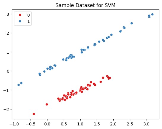
Let's consider a simple example dataset for binary classification - a set of points in a 2D space, each belonging to either class A or class B. Our goal is to train an SVM model to accurately classify new points into these two classes.
Sample Dataset:
| Feature 1 | Feature 2 | Class |
| 2 | 3 | A |
| 1 | 4 | A |
| 3 | 3.5 | B |
| 4 | 2 | B |
SVM Workflow:
Step 1: Load and Visualize the Dataset:
import matplotlib.pyplot as plt
import seaborn as sns
from sklearn.datasets import make_classification

# Create a sample dataset
X, y = make_classification(n_samples=100, n_features=2, n_classes=2, n_clusters_per_class=1, n_redundant=0, random_state=42)

# Visualize the dataset
sns.scatterplot(x=X[:, 0], y=X[:, 1], hue=y, palette="Set1")
plt.title("Sample Dataset for SVM")
plt.show()
Step 2: Train the SVM Model:
from sklearn.svm import SVC

# Create and train the SVM model
svm_model = SVC(kernel='linear')  # Linear kernel for simplicity
svm_model.fit(X, y)
Step 3: Visualize the Decision Boundary:
# Visualize the decision boundary
plt.figure(figsize=(8, 6))
sns.scatterplot(x=X[:, 0], y=X[:, 1], hue=y, palette="Set1")
ax = plt.gca()
xlim = ax.get_xlim()
ylim = ax.get_ylim()
# Create grid to evaluate model
xx, yy = np.meshgrid(np.linspace(xlim[0], xlim[1], 100), np.linspace(ylim[0], ylim[1], 100))
Z = svm_model.decision_function(np.c_[xx.ravel(), yy.ravel()])
# Plot decision boundary and margins
Z = Z.reshape(xx.shape)
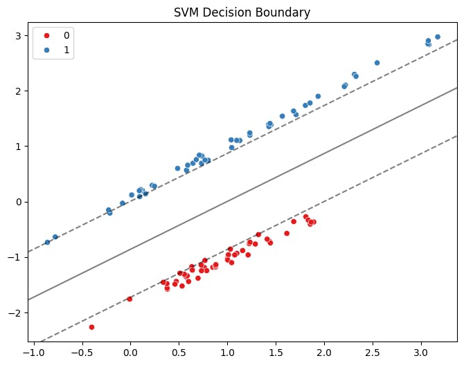
plt.contour(xx, yy, Z, colors='k', levels=[-1, 0, 1], alpha=0.5, linestyles=['--', '-', '--'])
plt.title("SVM Decision Boundary")
plt.show()
Code Explanation:
We create a sample dataset using
make_classificationwith two features and two classes.The dataset is visualized using a scatter plot.
An SVM model with a linear kernel is trained on the dataset.
The decision boundary of the SVM model is visualized, showcasing how it separates the two classes.
Certainly! Let's consider another example with a different dataset, visualization, and prediction using Support Vector Machines (SVM).
Example with the Iris Dataset:
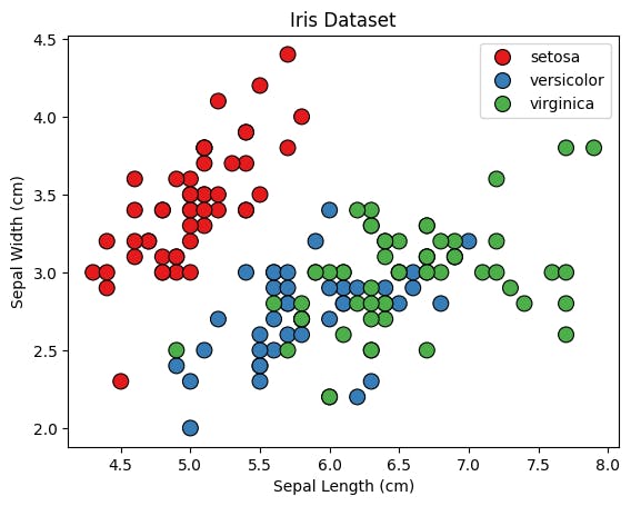
We will use the famous Iris dataset, which consists of three classes of iris flowers (setosa, versicolor, and virginica) based on four features (sepal length, sepal width, petal length, and petal width).
Here's a sample representation of the Iris dataset :
| Sepal Length (cm) | Sepal Width (cm) | Petal Length (cm) | Petal Width (cm) | Class |
| 5.1 | 3.5 | 1.4 | 0.2 | Setosa |
| 4.9 | 3.0 | 1.4 | 0.2 | Setosa |
| 7.0 | 3.2 | 4.7 | 1.4 | Versicolor |
| 6.4 | 3.2 | 4.5 | 1.5 | Versicolor |
| 6.3 | 3.3 | 6.0 | 2.5 | Virginica |
| 5.8 | 2.7 | 5.1 | 1.9 | Virginica |
| ... | ... | ... | ... | ... |
This table represents a subset of the Iris dataset, containing the sepal length, sepal width, petal length, petal width measurements for several iris flowers, along with their corresponding class labels (Setosa, Versicolor, Virginica). Each row in the table represents a single iris flower, and each column represents a specific attribute of the flower. This tabular representation allows for easy visualization and understanding of the dataset's structure and contents.
# Import necessary libraries
import numpy as np
import matplotlib.pyplot as plt
import seaborn as sns
from sklearn import datasets
from sklearn.model_selection import train_test_split
from sklearn.svm import SVC
from sklearn.metrics import accuracy_score, confusion_matrix
# Load the Iris dataset
iris = datasets.load_iris()
X = iris.data[:, :2] # Consider only the first two features for simplicity
y = iris.target
# Visualize the dataset
sns.scatterplot(x=X[:, 0], y=X[:, 1], hue=iris.target_names[y], palette="Set1", edgecolor='k', s=100)
plt.title("Iris Dataset")
plt.xlabel("Sepal Length (cm)")
plt.ylabel("Sepal Width (cm)")
plt.show()
# Split the dataset into training and testing sets
X_train, X_test, y_train, y_test = train_test_split(X, y, test_size=0.2, random_state=42)
# Create and train the SVM model
svm_model = SVC(kernel='linear', C=1) # Linear kernel with regularization parameter C=1
svm_model.fit(X_train, y_train)
# Visualize the decision boundary
plt.figure(figsize=(8, 6))
sns.scatterplot(x=X[:, 0], y=X[:, 1], hue=iris.target_names[y], palette="Set1", edgecolor='k', s=100)
ax = plt.gca()
xlim = ax.get_xlim()
ylim = ax.get_ylim()
# Create grid to evaluate model
xx, yy = np.meshgrid(np.linspace(xlim[0], xlim[1], 100), np.linspace(ylim[0], ylim[1], 100))
Z = svm_model.predict(np.c_[xx.ravel(), yy.ravel()])
# Plot decision boundary
Z = Z.reshape(xx.shape)
plt.contourf(xx, yy, Z, cmap=plt.cm.Paired, alpha=0.8)
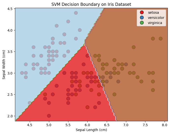
plt.title("SVM Decision Boundary on Iris Dataset")
plt.xlabel("Sepal Length (cm)")
plt.ylabel("Sepal Width (cm)")
plt.show()
# Make predictions on the test set
y_pred = svm_model.predict(X_test)
# Evaluate the model's accuracy
accuracy = accuracy_score(y_test, y_pred)
conf_matrix = confusion_matrix(y_test, y_pred)
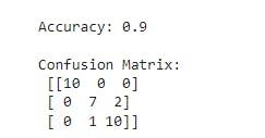
print("Accuracy:", accuracy)
print("\nConfusion Matrix:\n", conf_matrix)
In this example, we load the Iris dataset, visualize it, create a linear SVM model, visualize its decision boundary, and make predictions on a test set. The output includes the accuracy of the model and a confusion matrix for further evaluation.
Let's break down the code step by step:
Import Necessary Libraries:
- We import required libraries such as NumPy for numerical computations, Matplotlib for visualization, Seaborn for enhanced plotting, and scikit-learn for machine learning functionalities.
Load the Iris Dataset:
- We load the famous Iris dataset using scikit-learn's
datasetsmodule. The dataset contains information about iris flowers, including sepal and petal measurements.
- We load the famous Iris dataset using scikit-learn's
Visualize the Dataset:
- We create a scatter plot to visualize the iris dataset, using the sepal length and sepal width as the x and y axes, respectively. Each data point is colored according to the class of iris flower it represents.
Split the Dataset:
- We split the dataset into training and testing sets using the
train_test_splitfunction from scikit-learn. This step allows us to train the model on a subset of the data and evaluate its performance on unseen data.
- We split the dataset into training and testing sets using the
Create and Train the SVM Model:
- We create an SVM model with a linear kernel using the
SVCclass from scikit-learn. The parameterC=1specifies the regularization strength. We then train the model using the training data.
- We create an SVM model with a linear kernel using the
Visualize the Decision Boundary:
- We plot the decision boundary of the SVM model on the same scatter plot as the dataset. The decision boundary separates the different classes of iris flowers based on the SVM model's predictions.
Make Predictions on the Test Set:
- We use the trained SVM model to make predictions on the test set (which the model hasn't seen before) using the
predictmethod.
- We use the trained SVM model to make predictions on the test set (which the model hasn't seen before) using the
Evaluate the Model's Accuracy:
- We calculate the accuracy of the SVM model by comparing its predictions on the test set with the actual labels. Additionally, we compute the confusion matrix to further assess the model's performance.
The code demonstrates the entire workflow of using SVM for classification, from loading the dataset to training the model, visualizing the decision boundary, making predictions, and evaluating the model's accuracy. This approach helps in understanding how SVM works and how it can be applied to real-world datasets like the Iris dataset.
Conclusion:
Support Vector Machines are versatile and effective algorithms, particularly suitable for problems with clear margins between classes. By understanding the basics, exploring example datasets, and implementing SVMs with code and visualizations, you've gained insights into how SVMs work and their application to real-world scenarios.
In practice, SVMs prove beneficial in various fields, such as image classification, text categorization, and bioinformatics. As you delve deeper into the world of machine learning, SVMs stand as a valuable tool in your toolkit for tackling classification challenges with precision and efficiency.